5.6. Deep Learning#
![]()
Stochastic gradient descent and the like.

5.6.1. Supervised Learning Setup#
From data, learn concept.
In the supervised learning setup, we have a large number of examples of inputs \(x\) and corresponding labels \(y\). We will often refer to the training dataset as \(D\), consisting of pairs \((x,y)\). The nature of the output labels \(y\) determine the type of learning problem we are dealing with:
Classification; If the labels \(y\) are discrete, we talk about a supervised classification problem. The prototypical example is classifying images as portraying either a cat or a dog: here the images are the inputs \(x\), and the output label \(y \in \{\text{cat},\text{dog}\}\).
Regression If the labels \(y\) are continuous, this is called a supervised regression problem. For example, predicting the blue-book value of a second-hand car based on its make, model, year, and miles driven.
Whether we are talking about classification or regression, the supervised leaning process normally follows these steps:
Define a model \(f\) and its parameters \(\theta\) that allow you to output a prediction \(\hat{y}\) from the input features \(x\): \begin{equation} \hat{y} = f(x; \theta) \end{equation}
Divide your data into training, validation, and test datasets. Typically, the largest portion of the data is used for training, while setting aside smaller validation and test portions of the data.
Train the model using the training data \(D_{\text{train}}\), while monitoring for “overfitting” on the validation dataset \(D_{\text{val}}\). We train by adjusting the parameters \(\theta\) to minimize a training loss, both of which we look at in more detail below.
After we decide to stop the training process, we typically test the model on the held-out dataset \(D_{\text{test}}\) that the training process has never seen, to get an independent assessment of how well the model will generalize towards new, unseen data.
Supervised learning is the staple of machine learning and its use has exploded in recent years to encompass almost any human economic activity, ranging from finance to healthcare and everything in between. Most recently the success of large language models is also based on supervised learning, where a transformer-based model is trained to predict the next word (or token) in a sequence, from very large textual datasets, a paradigm which is rapidly finding its way to different modalities like vision as well.
5.6.2. Example: Interpolation in 1D#
As an example, we formulate a simple regression problem that asks for interpolating functions in 1D. We will create a differentiable interpolation scheme that can be trained using samples from any function we want to interpolate, even functions with multi-dimensional outputs.
The LineGrid class below is designed for this purpose, and divides up the 1D interval over which the function is defined in a number of cells, arranged in a 1D grid. It is initialized with two parameters:
n: the number of cells in a 1D gridd: the dimensionality of the function we want to interpolate
In our case, we will focus on interpolating the grid values defined at the cell boundaries. The forward method of the LineGrid module performs the interpolation for any value inside the grid.
def interpolate(v0, v1, alpha):
    """Interpolate between v0 and v1 using alpha, using unsqueeze to properly handle batches."""
    return v0 * (1 - alpha.unsqueeze(-1)) + v1 * alpha.unsqueeze(-1)

class LineGrid(nn.Module):
    """A 1D grid with learnable values at the boundaries on n cells."""

    def __init__(self, n, d=1):
        super().__init__()  # Calling the superclass's __init__ method
        self.grid = nn.Parameter(nn.init.normal_(torch.empty(n + 1, d)))

    def forward(self, x):
        X = torch.floor(x).long()
        a = x - X  # blending weights (same size as x)
        return interpolate(self.grid[X], self.grid[X + 1], a)
Here is an example of how to initialize a LineGrid instance, and subsequently call its forward method:
grid_module = LineGrid(n=5, d=2)

x = torch.Tensor([1.5, 2.7, 3.6])
print("Interpolated Output:", grid_module(x))
Interpolated Output: tensor([[-1.0894,  0.5480],
        [-0.8016, -0.6580],
        [ 0.2066,  0.5187]], grad_fn=<AddBackward0>)
In the example above, the shape of the output is \(3\times 2\) because we asked to interpolate a 2D function (d is 2) at three different locations (as x.shape is (3,)). In addition, the interpolate function is written to accommodate and shape for the tensor x to allow evaluating over arbitrary batches of examples. If we input a tensor with shape (b, m), the output will have shape (b, m, d), and so forth.
The output looks rather random, however, because the grid was initialized with random values in the constructor. Below we discuss often-used loss functions and the stochastic gradient descent method to train models, and show how to train the simple regression example above to drive all these concepts home.
5.6.2.1. Exercise#
For the example above with \(n=5\) and \(d=2\), give a single \((x,y)\) pair. What is the model \(f\)? What are the model parameters \(\theta\)? How many parameters are there?
5.6.3. Loss Functions#
A loss function for every occasion.
Different tasks require different loss functions, and a lot of creativity and research goes into crafting loss functions for complex tasks. For “vanilla” regression tasks, we typically use a mean squared error loss function as we already encountered before:
Above \(f(x;\theta)\) is the continuous prediction function implemented by, say, a neural network, where \(\theta\) represents the weights in all layers. Note that the formula above can be easily generalized to vector-valued labels \(y\). In fact, our 1D interpolation example above yielded a 2-dimensional output, so let us illustrate the MSE loss in that case:
label = torch.Tensor([[1.0, 2.0], [3.0, 4.0], [5.0, 6.0]])
print("Our MSE Loss:", ((grid_module(x) - label)**2).mean().item())
Our MSE Loss: 15.940658569335938
We used the vectorized versions of subtraction and power above, and then used the mean method of tensors. As you can see, the MSE loss in this case is 13.045638. Even though in this case the calculation is simple, many other loss functions exist and might not be as straightforward to implement. Luckily, PyTorch has many loss functions built-in:
mse = nn.MSELoss() # Instantiate the loss function
mse_loss = mse(grid_module(x), label) # Compute the loss
print("Pytorch MSE Loss:", mse_loss.item())
Pytorch MSE Loss: 15.940658569335938
For classification, the cross entropy loss function is very popular. It measures the average disagreement of the predicted labels with the ground truth labels:
This formula seems perhaps unintuitive and rather complicated; however, it is actually quite intuitive once you understand a few concepts. In particular, in the multi-class classification problem we assume that the model outputs a probability \(p_c(x;\theta)\) for every class \(c\in[N]\), where \(N\) is the number of classes. The quantity
is called the surprise that we should experience when seeing a label \(y=c\). Indeed, for example, if we see class \(3\) and the probability output by the network is \(p_3(x;\theta)=1\), we are not surprised at all, as \(\log\frac{1}{1}=\log 1 = 0\). However, if the probability is only \(0.01\), our surprise is \(\log\frac{1}{0.01}=\log 100 = 2\). The lower the probability, the higher the surprise. Hence, the cross-entropy above measures the average surprise for seeing the labeled examples in the training data. After training, the model is the least surprised possible, hopefully, which is why it is an intuitive loss function to minimize.
Note that training with cross-entropy does not guarantee that the outputs can be truly interpreted as probabilities: the recent field of model calibration has shown that especially neural networks can severely over-estimate those probability values in attempting to minimize the loss. If this interpretation is important for the application at hand, several techniques now exist to calibrate the models to be more interpretable that way.
5.6.4. Gradient Descent#
Calculate gradient, reduce loss.
A neural network output, and in particular a CNN, depends on the large set of continuous weights \(W\) that make up its convolutional layers, pooling layers, and fully connected layers. In other words, the neural network is the model \(f(x;\theta)\) in the learning setup discussed above, and the weights \(W\) are its parameters \(\theta\).
When we train a neural networks, we adjust its weights \(W\) to perform better on the task at hand, be it classification or regression. To measure whether the model performs “better”, we can use one of the loss functions defined above. To adjust the weights, we could calculate the gradient of the loss function with respect to each of the weights, and adjust the weights accordingly. That procedure is called gradient descent.
Below we illustrate gradient descent with the 1D interpolation model we created above. As an example, maybe we can learn a sine and cosine function at the same time? Let us create some training data by creating 500 noisy samples of these two functions. To integrate smoothly with the pytorch library we will use, we create a TensorDataset below.
m = 250  # number of samples to train our model
n = 20  # Grid size of 20, allowing for x values between 0 and 20
x_samples = torch.rand((m, )) * n
noisy_sin = torch.sin(x_samples * 2 * torch.pi / n) + 0.1 * torch.randn((m, ))
noisy_cos = torch.cos(x_samples * 2 * torch.pi / n) + 0.1 * torch.randn((m, ))
y_samples = torch.stack([noisy_sin, noisy_cos], dim=1)
dataset = TensorDataset(x_samples, y_samples)
A TensorDataset is a PyTorch class that wraps a pair of tensors, and its __getitem__ method retrieves a training sample by indexing the tensors along the first dimension. For example, we can retrieve the training sample with index 12, or even slice to get the 5 training samples with indices 10..14:
print("dataset[12]:", dataset[12])
print("dataset[10:15]:", dataset[10:15])
dataset[12]: (tensor(18.4051), tensor([-0.6276,  0.7498]))
dataset[10:15]: (tensor([ 6.1938,  2.6900, 18.4051, 10.2891, 11.0168]), tensor([[ 0.7433, -0.2394],
        [ 0.8976,  0.7410],
        [-0.6276,  0.7498],
        [-0.0018, -0.9387],
        [-0.4760, -0.9144]]))
We can then use the PyTorch training code below, which is a standard way of training any differentiable function, including our LineGrid class. That is because all the operations inside the LineGrid class are differentiable, so gradient descent will just work.
Inside the training loop below, you’ll find the typical sequence of operations: zeroing gradients, performing a forward pass to get predictions, computing the loss, and doing a backward pass to update the model’s parameters. Try to understand the code, as this same training loop is at the core of most deep learning architectures. Now, let’s take a closer look at the code itself, which is extensively documented for clarity, and listed in Figure 2.
#| caption: Code to train a model using gradient descent.
#| label: code:train_gd
def train_gd(model, dataset, loss_fn, callback=None, learning_rate=0.5, num_iterations=301):
    # Initialize optimizer
    optimizer = optim.SGD(model.parameters(), lr=learning_rate)

    # Extract data from dataset
    x_samples, y_samples = dataset[:]

    # Loop over the dataset multiple times (each loop is an iteration)
    for iteration in range(num_iterations):
        # Zero the parameter gradients
        optimizer.zero_grad()

        # Forward pass: Compute predicted y by passing x_samples through the model
        output = model(x_samples)

        # Compute loss
        loss = loss_fn(output, y_samples)

        # Backward pass and update
        loss.backward()
        optimizer.step()

        # Report if callback is given
        if callback is not None:
            callback(iteration, model)
To use the code, we initialize the model, specify the loss function, and create a callback function that allows us to monitor the progress made by the optimizer. After that, we simply call train_gd:
# Initialize model
model = LineGrid(n=n, d=2)  # d=2 as we are regressing both sin and cos

# Initialize the built-in Mean-Squared Error loss function
mse = nn.MSELoss()

# Create a callback that saves loss to a dataframe
loss_data = pd.DataFrame(columns=['Iteration', 'Loss'])
def record_loss(iteration, model):
    loss_data.loc[len(loss_data)] = [iteration, mse(model(x_samples), y_samples).item()]

# Run the training loop
train_gd(model, dataset, loss_fn=mse, callback=record_loss)
#| caption: Loss of the model during training. The loss decreases as the model learns to fit the data.
#| label: fig:loss_training
px.line(loss_data, x='Iteration', y='Loss')
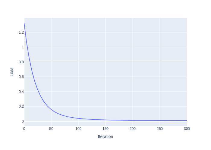
The resulting loss function is shown in Figure 2. Note that gradient descent converges rather slowly. You could try experimenting with the learning rate to speed this up.
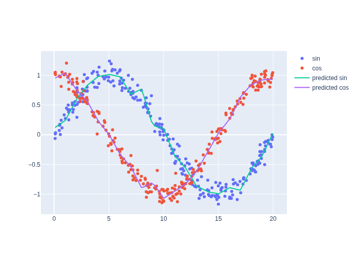
After the training has converged, we can evaluate the resulting functions and plot the result against the training data, and Figure 3 that we get decent approximations of sin and cos, even with noisy training data.
#| caption: Learned approximation of the sine and cosine functions. The model has learned to fit the data.
#| label: fig:sin_cos_approx
x_sorted = torch.sort(x_samples).values
y_pred = model(x_sorted).detach().numpy()
fig = plotly.graph_objects.Figure()
fig.add_scatter(x=x_samples, y=y_samples[:, 0], mode='markers', name='sin')
fig.add_scatter(x=x_samples, y=y_samples[:, 1], mode='markers', name='cos')
fig.add_scatter(x=x_sorted, y=y_pred[:, 0], mode='lines', name='predicted sin')
fig.add_scatter(x=x_sorted, y=y_pred[:, 1], mode='lines', name='predicted cos');
fig.show()
5.6.5. Stochastic Gradient Descent#
Stochastic gradient descent or SGD is an approximate gradient descent procedure, to cope with the very large data sets typically thrown at supervised problems. It is typically impossible to calculate the exact gradient, which requires looping over all the examples, which can run in the millions. An easy approximation scheme is to randomly sample a small subset of the examples, and calculate the gradient of the weights using only those examples. The upside is that this is much faster, but the downside is that this is only approximate. Hence, if we adjust weights with this approximate gradient, we might or might not make progress on the task. This procedure is called stochastic gradient descent, and it works amazingly well in practice.
The DataLoader class in PyTorch makes implementing SGD very easy: it can wrap any Dataset instance, and then retrieves training samples one “mini-batch” at a time. The code below uses a mini-batch size of 25, but feel free to experiment with different values for both this parameter and the learning rate to get a feel for what happens. Note that by convention we refer to one execution of the inner loop below, over a mini-batch, as an “iteration”. One full cycle through the dataset by randomly selecting mini-batches is referred to as an “epoch”.
def train_sgd(model, dataset, loss_fn, callback=None, learning_rate=0.5, num_epochs=31, batch_size=25):
    # Initialize optimizer
    optimizer = optim.SGD(model.parameters(), lr=learning_rate)

    # Create DataLoader for batch processing
    data_loader = DataLoader(dataset, batch_size=batch_size, shuffle=True)

    # Loop over the dataset multiple times (each loop is an epoch)
    for epoch in range(num_epochs):
        for x_batch, y_batch in data_loader:
            optimizer.zero_grad()
            output = model(x_batch)
            loss = loss_fn(output, y_batch)
            loss.backward()
            optimizer.step()

        if callback is not None:
            callback(epoch, model)
# Initialize model
model = LineGrid(n=n, d=2)  # d=2 as we are regressing both sin and cos

# Initialize the built-in Mean-Squared Error loss function
mse = nn.MSELoss()

# Create a callback that saves loss to a dataframe
loss_data = pd.DataFrame(columns=['Epoch', 'Loss'])
def record_loss(epoch, model):
    loss_data.loc[len(loss_data)] = [epoch, mse(model(x_samples), y_samples).item()]

# Run the training loop
train_sgd(model, dataset, loss_fn=mse, callback=record_loss)
#| caption: Loss of the model during stochastic gradient descent training.
#| label: fig:loss_training_sgd
px.line(loss_data, x='Epoch', y='Loss')

The training loss is shown in Figure 4. Note that we converge much faster in this case: in just 30 iterations we reached the same low loss as with 300 iterations before. The answer is because with 250 training samples and mini-batches of size 25, each epoch adjusts the model’s parameters 10 times. This effectively boosts the learning rate by a factor of 10. However, note that because each mini-batch looks at only one 10th of the dataset, each mini-batch’s adjustment could adversely affect the performance on the other training samples.
5.6.5.1. Validation and Testing#
In practice, validation and test datasets are used to evaluate the performance of a model. The validation dataset is used to tune the hyperparameters of a model, while the test dataset is used to evaluate the performance of the model on unseen data.
5.6.6. Transformer Architectures#
We would be remiss in not mentioning the increasing importance of transformer architectures in computer vision and robotics. A transformer network can be viewed as deep multi-layer neural network whose connections can be rewired during training, through a process called attention. This architecture has led to the breakthrough of large language models or LLMs, which take a large context of tokens and produce a next-token probability distribution , which is then sampled to output a response to an input prompt.
In computer vision, vision transformers or VITs use this same architecture, by tokenizing an image and provide it as part of the context. This allows LLM-style models to then answer questions about images, or perform traditional computer vision tasks such as object detection, image segmentation, and much more.
One step beyond VITs are vision-language-action models, specifically crafted for use in robots. They take not only visual input alongside language prompts, but also other signals such as joint angles (in case of articulated robotics), orientation sensors, etc… And, more importantly, they are trained to also output actions via specialized output heads, matched to the particular robot architecture that is targeted.
A drawback of transformer-based methods is that they take a large aount of time and effort to train, and running the models on embedded computers is also a challenge. Hence, convolutional architectures remain competetive in robotics, especially when computational resources are constrained and/or there are constraints on communication that prevent calling a remote API. However, this is an intense area of study and the mix between fully connected, convolutional, and transformer architectures is sure to shift.
While we do not discuss transformer architectures in detail here, some pointers into the literature are provided in section 5.7.